Contents
|
STG top Introduction How to make STG
Download STG Optimal schedules Links |
This page describes how to make task graphs in the STG. Currently, Standard Task Graph Set Archive consists of task graphs generated randomly and modeled from actual application programs without communication costs (i.e., 0 communication costs) as the first step. Task graphs with communication costs are forthcoming.
Task Graphs Generated Randomly
This section describes how we generated the 900 random task graphs in the Standard Task Graph Set. The graph sizes (in number of tasks) varies between 50 and 2700, such as 50, 100, 300, 500, 700, 900, 1100, 1300, 1500, 1700, 1900, 2100, 2300, 2500, and 2700.
Graph shapes (precedence constraints) were determined based on four different reported methods [V.Almeida92], [T.Yang94], [T.Adam74].
In the following, let A denote a task connection matrix with elements a(i,j), where i, 0<= i<=n+1, and j, 0<=j<=n+1, represent the task number (T0 is the entry dummy node and Tn+1 is the exit dummy node). When a(i,j)=1, task Ti precedes task Tj. In other words, Ti must be completed before the execution of Tj is started. On the other hand, when a(i,j)=0, Ti and Tj are independent of each other.
In the ``sameprob'' edge connection method [V.Almeida92], a(i,j) is determined by independent random values defined as follows:
where p indicates the probability that there exists an edge (precedence constraint) between Ti and Tj.
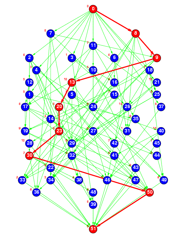
Figure 2(a) : sameprob
Figure 2(a) represents a random task graph having 50 tasks generated by the ``sameprob'' method, where the edge connection probability (p) was specified as 0.1. In the current STG, p is specified as 0.1 and 0.2.
However, with the ``sameprob'' method, the number of predecessors increases with the number of tasks. Therefore, the STG also uses another predecessor specification method, ``samepred''. The ``samepred'' method specifies the average number of predecessors for each task.
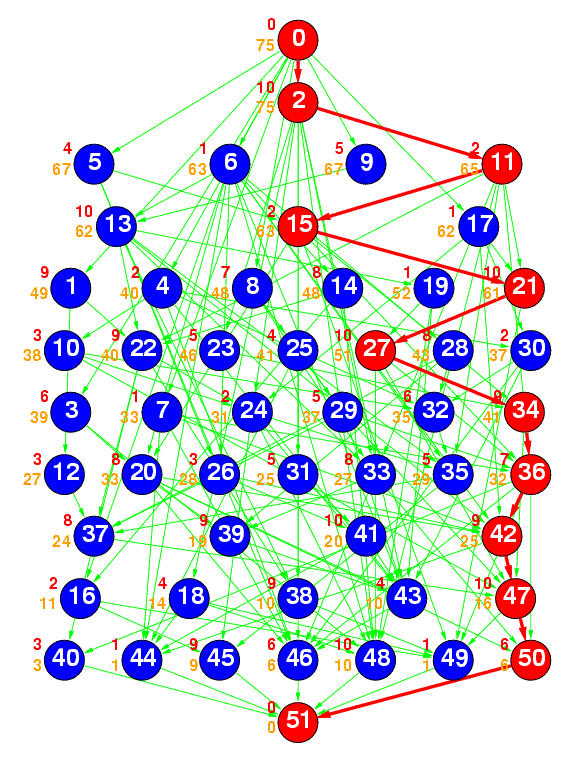
Figure 2(b) : samepred
Figure 2(b) represents a random task graph having 50 tasks generated by the ``samepred'' method, where the average number of predecessors was specified as 3. Currently, the average number of predecessors was set to 1, 3, and 5.
In another method, ``layrprob'' [T.Yang94], first the number of layers in the task graph is generated. Next, the number of independent tasks in each layer is randomly decided. Finally, edges between layers are connected with the same probability p as is ``sameprob''.
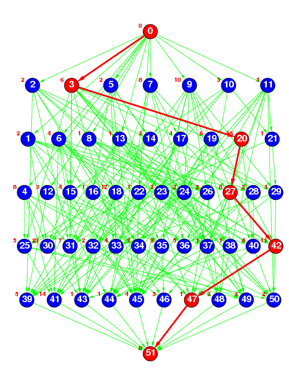
Figure 2(c) : layrprob
Figure 2(c) represents a random task graph having 50 tasks generated by the ``layrprob'' method, where the number of layers was specified as 5 and edge connection probability p was specified as 0.2. Currently, the average width of each layer (the average number of tasks in each layer) is fixed at 10, and the number of layers is calculated by (number of tasks)/10.
The last method ``layrpred'' generates layers in the same way as with ``layrprob'' and connects edges in the same way as with ``samepred''.
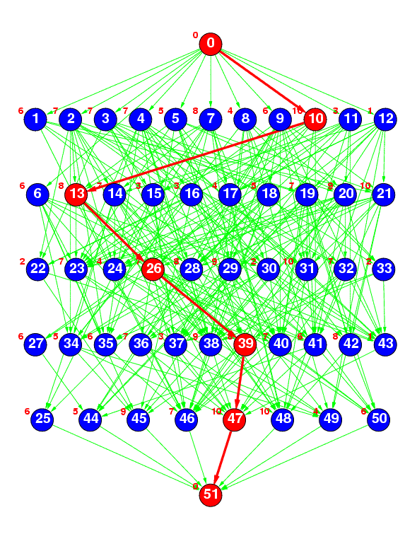
Figure 2(d) : layrpred
Figure 2(d) represents a random task graph having 50 tasks generated by the ``layrpred'' method, where the number of layers was specified as 5 and the average number of predecessors was specified as 5. Currently, the average width of each layer is fixed at 10, the number of layers is calculated by (number of tasks)/10, and the average number of predecessors is set to 1, 3, or 5.
The processing time of each task was determined using three methods. The mean value of the task processing time was fixed at 5 or 10 units of time [u.t.], and the processing time of each task was determined using uniformly distributed random numbers from 1 to 10[u.t.] (mean task processing time of 5[u.t.]) or from 1 to 20[u.t.] (mean task processing time of 10[u.t.]) [T.Adam74]; using exponentially distributed random numbers [V.Almeida92]; or using normally distributed random numbers with standard deviation of 1 (mean task processing time of 5[u.t.]) or 3 (mean task processing time of 10[u.t.]). These task processing time generation methods are identified using the names ``unifproc'', ``expoproc'', and ``normproc'', respectively, in each task graph file.
We can thus select from 15 different task numbers, 10 edge connection methods (precedence constraints form and average number of predecessors), 3 task processing time generation methods, and 2 average task processing times. The result is 900 possible task graphs.
Task Graphs Generated from Actual Application Programs
We previously proposed a Fortran multigrain parallelization compilation method and have been developing the OSCAR FORTRAN Compiler [H.Kasahara90], [H.Kasahara91], [A.Yoshida96].
The STG includes several task graphs of actual application programs generated by this compiler. Also, previously reported task graphs modeled from actual application programs [H.Kasahara85] are available. The current STG includes task graphs for robot control (Figure 3(a)), a sparse matrix solver (Figure 3(b)), and a part of fpppp in the SPEC benchmarks (Figure 3(c)).
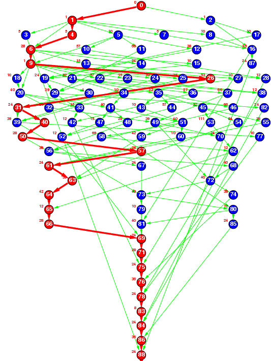
Figure 3(a) : Robot control
Figure 3(a) represents a task graph for Newton-Euler dynamic control calculation for the 6-degrees-of-freedom Stanford manipulator [H.Kasahara85].
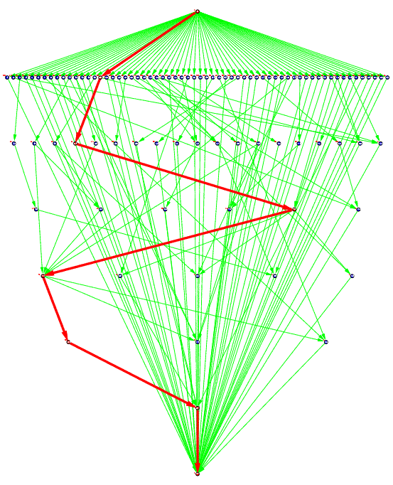
Figure 3(b) : Sparse matrix solver
Figure 3(b) represents a task graph for a random sparse matrix solver of an electronic circuit simulation that was generated using a symbolic generation technique and the OSCAR FORTRAN compiler (with actual execution cost of a multiprocessor system OSCAR).
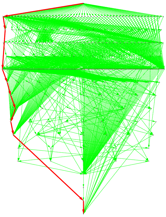
Figure 3(c) : SPEC fpppp
Figure 3(c) represents a task graph for subroutine fpppp, which is part of the SPEC benchmarks fpppp.
References
- [V.Almeida92] V. A. F. Almeida, I. M. M. Vasconcelos, J. N. C. Árabe and D. A. Menascé, "Using Random Task Graphs to Investigate the Potential Benefits of Heterogeneity in Parallel Systems", Proc. Supercomputing '92, pp. 683-691 (1992).
- [T.Yang94] T. Yang and A. Gerasoulis, "DSC : Scheduling Parallel Tasks on an Unbounded Number of Processors", IEEE Trans. Parallel and Distributed Systems, Vol.5, No.9, pp. 951-967 (1994).
- [T.Adam74] T. L. Adam, K. M. Chandy and J. R. Dickson, "A Comparison of List Schedules for Parallel Processing Systems", Communications of the ACM, Vol.17, No.12, pp. 685-690 (1974).
- [H.Kasahara90] H. Kasahara, H. Honda and S. Narita, "Parallel Processing of Near Fine Grain Tasks Using Static Scheduling on OSCAR", Proc. IEEE ACM Supercomputing '90 (1990).
- [H.Kasahara91] H. Kasahra, H. Honda, A. Mogi, A. Ogura, K. Fujiwara and S. Narita, "A Multi-grain Parallelizing Compilation Scheme for OSCAR", Proc. 4th Workshop on Languages and Compilers for Parallel Computing (1991).
- [A.Yoshida96] A. Yoshida, K. Koshizuka and H. Kasahara, "Data-Localization for Fortran Macrodataflow Computation Using Partial Static Task Assignment", Proc. 10th ACM Int'l Conf. on Supercomputing, pp. 61-68 (1996).
- [H.Kasahara85] H. Kasahara and S. Narita, "Parallel Processing of Robot-Arm Control Computation on a Multiprocessor System", IEEE J. Robotics and Automation, Vol.RA-1, No.2, pp. 104-113 (1985).
|
|
|
|